Baseball Statistics with R – Batting Average

I'm working on a new book about the R programming language. R is a language that is designed for use with statistics and data. I use it to analyze sports and social networking. I thought that it would be fun to write the book focusing on baseball statistics using data from Major League Baseball.

This post pulls the Batting Average topic from the book. I’ll try to provide enough information to get you started if you’re new to R. The book will include a tutorial and information about the R language.

Statistics in baseball can run from the very simple to the very complex. The complex end of the spectrum leads into the more advanced field of sabermetrics. Some of the advanced sabermetric calculations can’t be done without access to proprietary databases, and so for the most part my book will focus on what we can figure out using the data that’s easily available.

Almost everything you want to know about baseball statistics is already available on the internet, sliced and diced for you from sites like Baseball Prospectus and Fangraphs. It’s a lot of fun though, to sift through the data yourself. R is a great laboratory for that.

To get started, you’ll need R and you’ll need the baseball database. I would also suggest getting an IDE to make your work easier. Here are some links to get started:

The Comprehensive R Archive Network – This is where you can download R for the platform of your choice.

SeanLahman.com -   Sean Lahman maintains Lahman’s Baseball Database, which includes data on Major League Baseball going back to 1871. For the samples I create, you’ll need the comma delimited version of the database. Unzip it to a convenient place on your PC and keep the path handy.

RStudio – There are a number of IDEs available for R, but my favorite is RStudio. This IDE makes it very easy to edit and run code, import .csv data into data frames, and to load R packages.

sqldf – sqldf is the package I use to run SQL statements on R data frames. There are a couple of different ways that you can access databases in R, but this one is very simple and it’s very easy to get up and running with it. By default sqldf uses SQLite on the backend, but it can be configured to use other database programs as well.

Install R and RStudio and spend some time on a couple of the tutorials available on the internet. Install the sqldf package and take a look at the documentation.

Finally unzip the baseball database to a convenient location on your computer.

The following is the Batting Average topic. I would appreciate feedback, so please feel free to leave a comment or drop me a note at brianjo@gmail.com.

Batting Average

Batting average is perhaps the best known of all baseball statistics. It’s a favorite of fans because it’s a simple calculation. A player’s batting average is calculated by dividing the number of Hits by the number of At Bats. This calculation does not count Walks, Sacrifice Flies, Sacrifice Hits, Hit by Pitch, or Catcher Interference.

Formula:

BA = H/AB

Batting average can be calculated for any arbitrary number of At Bats, but it is generally used to describe batting performance over a series, a streak, a season, or a career.

Let’s take a look at how to calculate batting average in R for a player over the course of a season and then do the same for a career.

First we need to load up two tables. The Master table will give us the details we need on the player and the Batting table will let us take a look at those statistics.

> Master <- read.csv("~/SkyDrive/Documents/Stats/Baseball/Master.csv")
> Batting <- read.csv("~/SkyDrive/Documents/Stats/Baseball/Batting.csv")

Tables in R are generally referred to as data frames. Now that we have some data frames loaded in, let’s narrow things down and get the statistics for the player we’re looking for. In this case, let’s take a look at how Ted Williams did in 1941. To do this we’ll perform two steps. First we need to get Ted Williams’ playerID from the Master table:

We’ll use sqldf for our query:

> library("sqldf", lib.loc="C:/Users/Brian/R/win-library/2.15")
> tedwill <- sqldf("SELECT playerID FROM Master WHERE nameLast='Williams' AND nameFirst='Ted'")

So now we have Ted Williams’ playerID in the value tedwill. We can use that in our code, but it’s just as easy in this case to take note of the actual ID and use it in our next query. So let’s pull Williams’ stats out of the Batting data:

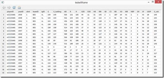
> tedwillframe <- sqldf("SELECT * from Batting WHERE playerID='willite01'")

This produces a nice table that contains Ted Williams’ career batting statistics.

Now that we’ve narrowed things down a bit, let’s calculate Ted’s batting average for 1941.

First, we’ll isolate the year we’re looking for:

> tedwill41 <- sqldf("SELECT * from tedwillframe WHERE yearID=1941")

Then we’ll perform a calculation based on the values for hits (H) and at bats (AB) for that year. Note that columns are accessed from the data frame with the $ character.

> tedwill41ave <- tedwill41$H/tedwill41$AB

We can type in tedwill41ave to see the result:

> tedwill41ave
[1] 0.4057018

Of course, batting averages are usually calculated to the hundredths place so we can round up the result in our query like so:

> tedwill41ave <- round(tedwill41$H/tedwill41$AB, digits=3)

Because we pulled Williams’ batting data into a single table, we can get his lifetime batting average by summing the Hits and the At Bats columns and performing our calculation. We’ll also use the round function and combine this all into a single command:

> tedwilllife <- round(sum(tedwillframe$H)/sum(tedwillframe$AB), digits=3)
> tedwilllife
[1] 0.344

As a quick review, for the lifetime average, we summed the column H from the table tedwillframe with sum(tedwillframe$H) and we did the same with the column AB. We divided H by AB and we wrapped all that in the round function which gave us the average rounded to 3 digits.

Finally, let’s create a new data frame that contains Ted Williams’ batting average year by year and chart the average.

R is really powerful in that you can perform calculations on vectors very easily. This means we can take a table full of batting data and perform all sorts of interesting calculations on the data.

> tedwillyby <- data.frame(tedwillframe$yearID, round((tedwillframe$H / tedwillframe$AB), digits=3))

In this case we created a new data frame containing the yearID in one column and the calculated batting average for that year in other.

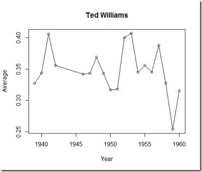
Finally, since we have the yearly batting average in a data frame, we can easily generate graphics based on that data. So let’s make a simple plot of the yearly data based on the tedwillyby data frame we just created.

> plot(tedwillyby, "o", main="Ted Williams", xlab="Year", ylab="Average")

It’s not a beautiful plot, but it will do for now. Ted Williams served as a Marine in two wars and his baseball career was interrupted. This graph could use an overlay that shows the years he played a shortened season, but I’ll save that for another post.